Partitioning variance between confounded fixed and random effects
One of my dissertation chapters assesses the habitat associations of wild bee species. My analysis to determine these habitat associations uses generalized hierarchical (or ’mixed effect’) linear models (i.e., GLMMs). The data consists of bee abundance across a number of sites, and landscape composition measured using remotely sensed data and GIS. My analytical approach is to model the observed abundance of a bee species at a site as a function of the habitat surrounding that site, as well as some covariates and random effects. Because sites were visited multiple times, one of the random effects is a random intercept for site. That is, my models look something like this: $$ bee ~ abundance \sim habitat + covariates + (1 | site) $$ I have published analyses using this sort of model before, and I see this sort of model used regularly, and so did not think too much about it. But, the first time I presented this analysis to my lab group, my advisor said, “But your habitat measurements don’t change between site visits, so how will the model know whether to attribute variance to habitat or the random effect?” Meaning: my habitat measures and random effects are confounded. How can I tell the difference?
I was shook.
Maybe someone with deeper knowledge of maximum likelihood methods would have been less phased. Surely other people have thought about this and the answer is out there. But I hadn’t encountered it, and so this sent me reeling. How would the model know the difference?
The problem of confounded predictors is a classic cautionary tale we all hear when learning statistics. Including co-linear predictors will reduce effect sizes and increase uncertainty. And the reason is pretty clear: if two predictors are correlated with each other and with the response variable, then the variance explained in the response could be attributed entirely to one and not at all to the second, or vice versa, or it could be split between them. As a result, the slope estimates tend to be smaller and their variances are inflated.
Is it any different when a predictor is confounded with a random effect? As it turns out, the answer is yes. I’ll demonstrate why.
To restate the question: How does a model partition variance between fixed and random effects? In a situation where a fixed-effect predictor is confounded with a random effect, such as the landcover around a series of sites with repeated visits, what is to keep a model from attributing the habitat effect to the site-level random effect?
The answer, in short, is that maximizing a model’s likelihood actually seems to require minimizing the variance of all random variables in the model. At least as much as possible without putting observations into the tails. As a result, a maximum likelihood algorithm will always attribute as much variance as possible to the fixed effects before attributing it to a random variable. In fact, at least in the simple examples I used to figure this out, including a random effect had no effect on the point estimate of the slope of the fixed effect.
To see why this is, let’s look at how likelihoods are calculated. The likelihood of a hierarchical (or mixed-effect) model is calculated as the product of probability density functions (see below for the math). Importantly, the probability density around the peak — that is, around the expected value — decreases as the variance of the density function increases. This is because the area under a probability density curve always sums to 1, which means that as a distribution gets broader (as it does with increasing variance), it also gets shorter.
The fact that probability density curves get lower as they get broader is key to fitting all random variables in a model. When fitting a residual variance term, this effect of variance on likelihood means a balance must be struck between keeping the variance high enough to keep observations out of the extremes of the tails, but not so high that the likelihood of the most common observations is depressed. If the residual variance term were too high, probability mass would get shifted into the empty tails of the distribution, and the absolute likelihood of the most common values would decrease, lowering the overall model likelihood. When fitting a random intercept term, this effect of variance on likelihood means there is an incentive to attribute variation among groups to fixed effects first; if the expected values of different groups can be made more similar by a linear combination of predictor variables, the variance of the random effect can be reduced, thereby increasing the likelihood of (at least most) site-level intercepts and therefore also the model as a whole.
To illustrate, first we’ll examine the probability density function for the normal distribution, then look at the mathematical likelihood statements for a simple hierarchical model, then simulate some data in R.
To see how this all works, we don’t actually need the full density function for the normal distribution, we can just look at its curve, plotted for a couple values of $\sigma$:
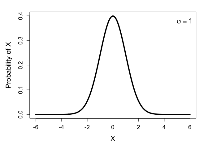
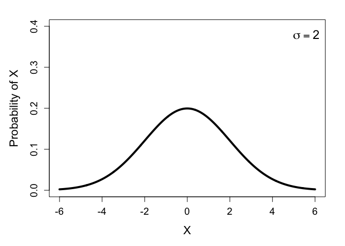
Notice how the distribution with higher variance is wider and shorter. This means the probability density of the most common values decrease when the variance is higher. (In fact, at least for the normal distribution, the probability of the expected value is perfectly inversely proportional to the variance: it halves when the variance is doubled, and doubles when the variance is halved. This is something I stumbled across while writing this.)
So, how does this play out when calculating the likelihood of a model? Let’s look at how model likelihoods are calculated. For the example above, regarding habitat predictors measured at the site level, the likelihood statement would look like this:
$$ L = P(\boldsymbol{y} | \boldsymbol{B}, \alpha, \epsilon, \sigma) = \Pi_i \Pi_j ~ N(y_{ij} | \beta_{0,i} + \beta_1 x_i, \epsilon) \times N(\beta_{0,i} | \alpha, \sigma) $$ where $y_{ij}$ is the $j$th observed response variable at site $i$, $\alpha$ is the grand mean (i.e., mean of site means), $\beta_{0,i}$ is the mean (or intercept) of site $i$, $\sigma$ is the standard deviation of site means, $\epsilon$ is the residual variation around site means, $\beta_1$ is the effect of the predictor variable $\boldsymbol{x}$, and $x_i$ is the habitat variable measured at site $i$. For simplicity, I excluded other covariates.
In this example, increasing $\sigma$ will decrease the probability density of $\boldsymbol{\beta_0}$. Thus, if differences among sites can be reduced by including the habitat predictor (through the linear combination $\beta_{0,i} + \beta_1 x_i$), then $\sigma$ can be reduced and the model likelihood will increase.
To demonstrate further, let’s consider some explicit, quantitative examples.
First, let’s consider the probability density for the expected value of a distribution, and how that changes as we increase the variance of its density function:
# observed value:
y = 0

# putative standard deviations:
sigma = seq(1, 10, 0.2)

#likelihood of expected (mean) value, given those sigmas:
L = dnorm(y, mean = y, sd = sigma, log = F)

# plot:
par(mar = c(5,6,2,2))
plot(sigma, L,
     xlab = "sd of random variable",
     ylab = "Probability density of \n of expected value",
     cex.lab = 1.5)
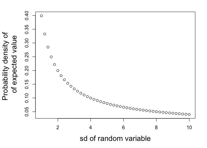
The larger the variance, the less probable the most common values…
Now let’s play with some data, and see how this affects model likelihoods.
To start, consider a non-hierarchical model, where we simply use likelihood to fit a variance parameter.
set.seed(42)
# true population parameters:
mu = 0
sigma = 1

# sample size:
n = 40

# observations
y = rnorm(n, mu, sigma)

# log likelihood of the true model:
ll_true = dnorm(y, mu, sigma) %>% prod %>% log
cat("true log-lik: ", ll_true)
## true log-lik: -65.92633
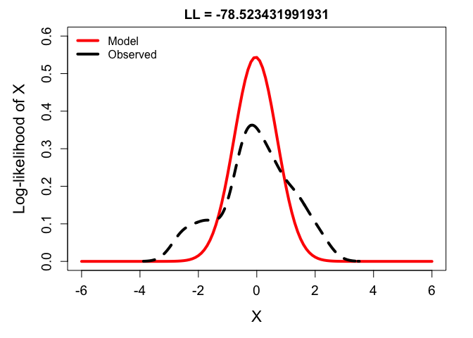
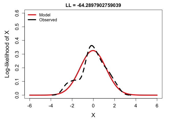
Now let’s look at the distributions described by different possible
variance parameters, and how these affect the likelihood of the implied
model. Below are density plots of y, which was randomly generated
above, overlaid with Normal density functions with three different
variances. The label at the top denotes the log-likelihood of the model
(i.e., the probability density of the observations, given that
particular normal distribution).
par(mar = c(5,5,2,2), cex.lab = 1.4, cex.axis = 1.2)
x = seq(-6,6,0.1)

# variance too low:
ll_low <- dnorm(y, mean(y), sd(y)*0.6) %>% prod %>% log
plot(x, dnorm(x, mean(y), sd = sd(y)*0.6), type ='l',
     main = paste0("LL = ", ll_low), xlab = "X", ylab = "Log-likelihood of X",
     ylim = c(0,0.6), lwd = 4, col = 'red')
lines(density(y), lwd = 4, lty = 2)
legend('topleft', bty = 'n',
       lwd = 4, col = c('red', 'black'), lty = 1,
       legend = c("Model", "Observed"))
# variance just right:
ll_goldi <- dnorm(y, mean(y), sd(y)) %>% prod %>% log
plot(x, dnorm(x, mean(y), sd = sd(y)), type = 'l',
     main = paste0("LL = ", ll_goldi), xlab = "X", ylab = "Log-likelihood of X",
     ylim = c(0,0.6), lwd = 4, col = 'red')
lines(density(y), lwd = 4, lty = 2)
legend('topleft', bty = 'n',
       lwd = 4, col = c('red', 'black'), lty = 1,
       legend = c("Model", "Observed"))
# variance too high:
ll_high <- dnorm(y, mean(y), sd(y*1.4)) %>% prod %>% log
plot(x, dnorm(x, mean(y), sd = sd(y)*1.4), type = 'l',
     main = paste0("LL = ", ll_high), xlab = "X", ylab = "Log-likelihood of X",
     ylim = c(0,0.6), lwd = 4, col = 'red')
lines(density(y), lwd = 4, lty = 2)
legend('topleft', bty = 'n',
       lwd = 4, col = c('black', 'red'), lty = 1,
       legend = c("Observed", "Model"))
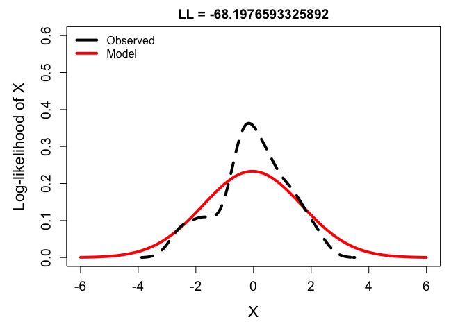
From these, you can see that the best balance is struck by fitting the density function to the frequency distribution of the observations. But just to drive it home, check out the likelihoods calculated across a range of possible variance parameters:
# possible sigmas:
sig.hat = seq(0.1, 5, 0.01)

# log likelihood of models using a range of possible sigmas:
ll_mod = purrr::map_dbl(sig.hat, function(sig){
  dnorm(y, mu, sig) %>% prod %>% log
})

# Most likely sigma?
ml.sig <- sig.hat[which.max(ll_mod)]
cat("most likely sigma: ", ml.sig)
## most likely sigma: 1.21
# plot LL against putative sigmas,
# w/ most likely value denoted by vertical line:
plot(sig.hat, ll_mod,
     xlab = expression(Putative~sigma), ylab = "Log-likelihood",
     cex.lab = 1.5, cex.axis = 1.2)
abline(v = ml.sig, col = 'red', lty = 2, lwd = 2)
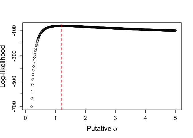
Here, low values of $\sigma$ are less likely because they put the observations into the tails of the distribution, while large values of $\sigma$ are less likely because they depress the probability density of even the most likely observations. The most likely value, then, is very close to the true population parameters. Which is all to say, it works as intended — whew!
So how does this all play out in the context of a hierarchical linear model? We’ll follow the example I start with, where we have repeated observations at a series of sites, and habitat, the predictor variable, is also measured at the level of the site. We’ll start with a scenario in which there is no true site effect, other than the effect of habitat, then we’ll build it out from there.
First we’ll simulate some data:
# simulated study design:
n_sites = 25
obs_per_site = 10
total_obs = n_sites*obs_per_site

# at which site was each observation taken?
site_id = rep(1:n_sites, each = obs_per_site)

# parameters:
grand_mean = 0
sd_residual = 1

# habitat data:
habitat = rnorm(n_sites)

# true effect of habitat:
beta = 2

# for data with no additional site effect:
site_means = grand_mean + habitat*beta

# observations:
y = rnorm(total_obs, mean = site_means[site_id], sd = sd_residual)
Now we’ll calculate the likelihood of a couple models of these data. In the first model, site variation is described with a fixed effect, like so: $$ L = P(\boldsymbol{y} | \alpha, \beta, \epsilon) = \Pi_i ~ N(y_i | \alpha + \beta * x_i, \epsilon) $$ where $y_i$ is the $i$th observation, $\alpha$ is the intercept, $\beta$ is the effect of the habitat predictor, and $\epsilon$ is the residual variance. In this model, the site-level expectation is determined by the combination of the single intercept and the fixed habitat effect. (Note: this model would not be appropriate because the repeated observations at a site is a form of pseudo-replication, but forget about that for now…)
In the second model, site variation is described with a random effect, like so: $$ L = P(\boldsymbol{y} | \boldsymbol{\beta}, \alpha, \epsilon, \sigma) = \Pi_i \Pi_j ~ N(y_{ij} | \beta_i, \epsilon) \times N(\beta_i | \alpha, \sigma) $$ where $y_{ij}$ is the $j$th observation at site $i$, $\beta_i$ is the expected value at site $i$, around which observations vary according to the residual variance parameter $\epsilon$. In turn, the site-level expectations, $\boldsymbol{\beta}$, vary around the grand mean, $\alpha$, according to the site-level variance parameter $\sigma$. Here, the site-level expectations $\boldsymbol{\beta}$ are the random effect.
We’ll see that avoiding random variables, when they aren’t needed, inherently increases the model likelihood.
# likelihood of fixed effect model
ll_fixed = dnorm(y, grand_mean + habitat[site_id]*beta, sd_residual) %>% prod %>% log

# likelihood of random effect model:
ll_random = log(
  prod(dnorm(y, site_means[site_id], sd_residual)) * # likelihood of observations, given site-level expectations
    prod(dnorm(site_means, grand_mean, sd(site_means))) # likelihood of those site-level expectations, given the grand mean
)

cat("Log likelihood of fixed effect model:", ll_fixed)
## Log likelihood of fixed effect model: -338.058
cat("Log-likelihood of random effect model", ll_random)
## Log-likelihood of random effect model -389.7722
Importantly, the fixed effect model does not perform better because it is the “true” model. Yes, the form of the model does match how we generated the data. But the random effect model is also “true” in that the expected values of the model are the true expected values that were used to generate the data. Check it out:
# left argument is expectation of fixed effect model,
# right argument is expectation of random effect model
all.equal((grand_mean + habitat[site_id]*beta), site_means[site_id])
## [1] TRUE
Next, to demonstrate that this works in real life, and that MLE
algorithms do indeed prefer the fixed effect components, we can fit
linear models like we would in real life, using lme4:
fm.null <- lm(y ~ 1)
fm.fixed <- lm(y ~ habitat[site_id])
fm.random <- lme4::lmer(y ~ 1 + (1|site_id), REML = F)
fm.mixed <- lme4::lmer(y ~ habitat[site_id] + (1|site_id), REML = F)
## boundary (singular) fit: see help('isSingular')
MuMIn::model.sel(fm.null, fm.fixed, fm.random, fm.mixed)
## Model selection table
##              (Int) hbt[sit_id]   class REML random df   logLik   AICc  delta
## fm.fixed  -0.02460       1.977      lm              3 -336.670  679.4   0.00
## fm.mixed  -0.02460       1.977 lmerMod    F    s_i  4 -336.670  681.5   2.07
## fm.random  0.05875             lmerMod    F    s_i  3 -388.110  782.3 102.88
## fm.null    0.05875                  lm              2 -541.006 1086.1 406.62
##           weight
## fm.fixed   0.737
## fm.mixed   0.263
## fm.random  0.000
## fm.null    0.000
## Abbreviations:
##  REML: F = 'FALSE'
## Models ranked by AICc(x)
## Random terms:
##  s\_i: 1 | site\_id
Note: these log-likelihood numbers don’t quite match mine, because they were calculated with fit model parameters, whereas I calculated likelihood with the true generating parameters. Also, it’s inappropriate to directly compare AICs of models with different fixed and random effect structures. But I think my point still stands.
As one final demonstration, let’s add a site-level effect that is separate from the habitat effect. This will mean that the “true” and best model will include both a site-level random effect and the site-level habitat effect. Can the model distinguish them?
# additional site variation:
sd_sites <- 1

# site means without habitat:
site_means = rnorm(n_sites, grand_mean, sd_sites)

# site means with habitat,
# which serve as statistical expectation at the site level:
linear_predictor <- site_means[site_id] + habitat[site_id]*beta

# observations:
y = rnorm(total_obs, mean = linear_predictor, sd = sd_residual)

# models:
fm.null <- lm(y ~ 1)
fm.fixed <- lm(y ~ habitat[site_id])
fm.random <- lme4::lmer(y ~ 1 + (1|site_id))
fm.mixed <- lme4::lmer(y ~ habitat[site_id] + (1|site_id))

MuMIn::model.sel(fm.null, fm.fixed, fm.random, fm.mixed)
## Model selection table
##              (Int) hbt[sit_id]   class random df   logLik   AICc  delta weight
## fm.mixed  -0.15160       1.739 lmerMod    s_i  4 -386.732  781.6   0.00      1
## fm.random -0.07825             lmerMod    s_i  3 -405.257  816.6  34.98      0
## fm.fixed  -0.15160       1.739      lm         3 -416.645  839.4  57.76      0
## fm.null   -0.07825                  lm         2 -540.068 1084.2 302.56      0
## Models ranked by AICc(x)
## Random terms:
##  s\_i: 1 | site\_id
As you can see, the algorithm does not sink all the variance into the random effect. In fact, if you look at the coefficient estimates, you’ll see that including the random effect has no effect whatsoever on the point estimate of the habitat effect.
And so it turns out we don’t need to worry about having confounded fixed and random effects. At least in this case. Which means my dissertation is safe. W00t ^_^